Primer of Phylogenetic Networks

*Editor’s Note: In “Genealogical Trees and Networks: Insights from Evolutionary Biology,” Ryan McDermott discusses the application of genealogical tree and network analogies in the humanities. He notes that while genealogical concepts are widely invoked in the historical disciplines, relatively few scholars have access to a robust background in genealogy proper. What follows here is a “Primer of Phylogenic Networks” by David Morrison, phylogeneticist and bioinformatician. You can see the following concepts at work in many articles in this journal, including McDermott’s follow-up essay, “Genealogies in Motion: Trees of Consanguinity.”

Introduction

Phylogenetic analysis is now widely used for comparative analyses in all areas of biology. Traditionally, these analyses have used trees to display their results, but in the last 30 years interest has developed in networks, which are a generalization of trees that can be used to investigate both vertical evolution (parent to offspring) and horizontal evolution (transfer among offspring).

In a study of a phylogenetic history, if there are no conflicting patterns of variation in the data then the traditional use of a phylogenetic tree is appropriate; but if there are apparently conflicting data patterns then a phylogenetic network will be more informative. It is necessary to distinguish two types of phylogenetic network, with the distinctly different objectives of displaying the data variation (data-display networks) versus analyzing the evolutionary history (evolutionary networks). The display networks are used for exploratory data analysis (EDA) while the evolutionary networks are used for formal phylogenetic analysis.

This primer presents a brief introduction to these two types of network, showing their relationship to each other, as well as to the original character data and the phylogenetic trees derived from those data. A small dataset from the literature is used for illustrative purposes.

I assume that you already have some familiarity with phylogenetic trees, and that you are interested primarily in expanding your knowledge to include networks.

The Data

Donoghue et al. (Systematic Botany 29:188-198, 2004) were interested in assessing the evolutionary relationships within the plant genus Viburnum, for which they sequenced 1,131 nucleotides of the chloroplast trnK intron and 556 nucleotides of the nuclear ribosomal Internal Transcribed Spacer (ITS). Five closely related species sampled from North America will be discussed here, as a simple but real dataset.

A summary of the nucleotide sequence data for the five species is shown in Figure 1. Each row in the alignment is a DNA sequence from one of the species, and each nucleotide position (column) along the sequence represents a character, with the different nucleotides in a column being different character states of the same character. All of the constant characters (i.e. the same nucleotide in all 5 of the sequences) have been deleted from the Figure (because they tell us nothing about the relationships among the species). Characters 1-12 are from the trnK gene and 13-43 are from the ITS gene (out of 1,131 and 556 nucleotides positions in the original gene sequences, respectively). Note that the data are strictly binary (i.e. no more than two character states per character), and so the data patterns are relatively straightforward.

Figure 1. The non-constant Viburnum characters. The vertical line separates the two genes.

We will first look at the use of networks for displaying these data and exploring the data patterns in the dataset, and then proceed to the use of networks for evolutionary analysis of the data.

Data Display and Exploration

Looking at a sequence alignment is a valuable way to view and understand the character data, since homologous states of the same character are aligned. The sequence of characters along the DNA can thus be easily compared across the rows, and the comparable character states at each DNA position can easily be compared down the columns.

So, in one important sense the sequence alignment is the phylogenetic data, expressed in a tabular format. However, the relationships among the taxa, whether phylogenetic or otherwise, are not necessarily easy to see from the alignment alone.

This can be addressed to some extent by uniquely coloring each nucleotide, as shown in Figure 2. This makes the comparison of the columns easier by providing visual clues about the patterns among the sequences. For example, it becomes obvious that positions 2 &11 have the same distribution of states among the sequences. However, it is not necessarily obvious that positions 7, 12, 13, 14, 15, 16, 19, 25, 28, 34, 36, 37, 38 & 43 also have this same distribution, because in these cases the pattern is formed by different color combinations.

Figure 2. The characters from Figure 1 with the nucleotides colored. The vertical line separates the two genes.

This issue could be addressed by re-arranging the columns so that similar patterns are adjacent, as shown in Figure 3. This indicates that the characters show 9 distinct patterns of relationship among the sequences, out of the 15 patterns possible. These patterns are supported by a wide variety of combinations of the four nucleotides, although 23 out of the 43 characters have C-T substitutions. Note, also, that this approach does lose the inherent order of the nucleotide positions (i.e. the characters are now unordered rather than ordered).

Figure 3. The characters from Figure 2 re-arranged into identical nucleotide patterns. The vertical lines separate the 9 character patterns.

A better visual display is to use a graph rather than a table, since graphs are designed specifically for visualizing data. Phylogeneticists have always used a connected line graph for this purpose, with the leaves labeled with the sequence names. Indeed, biologists used such graphs even before mathematicians developed modern graph theory. A leaf-labeled connected line graph is, in our terminology, a network. The edges (the lines) connect nodes together, some of the nodes representing the sequences and others possibly representing inferred ancestors, with every sequence being connected to every other sequence via some combination of edges and nodes.

Networks

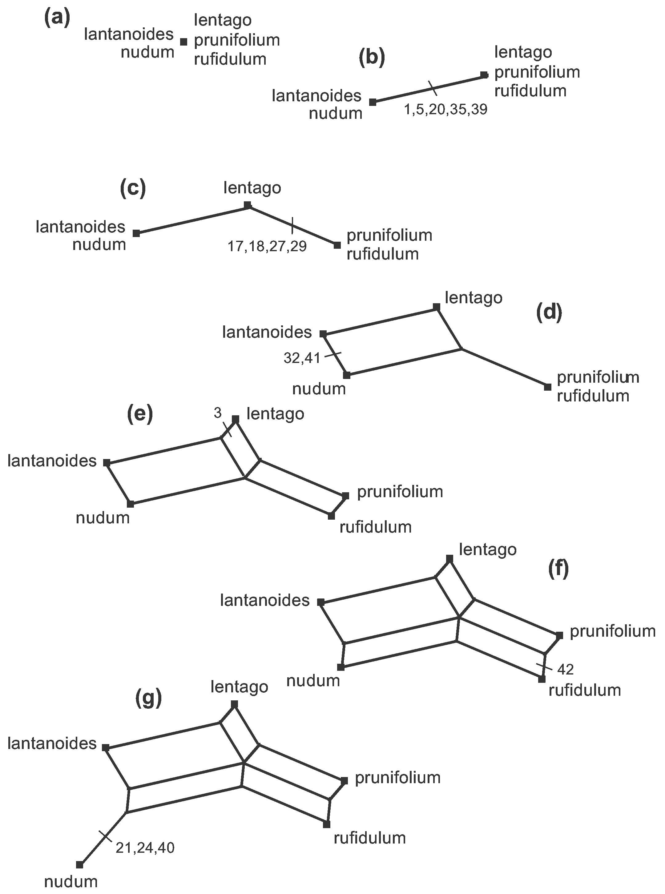
One simple type of line graph that is suitable for phylogenetics is a Splits Graph. The one shown here is called a Median Network, which can easily be derived directly from the unordered character data, as shown step by step in Figure 4. This figure is also available as an animation (click to open the animation is a new window—the animation loops indefinitely).

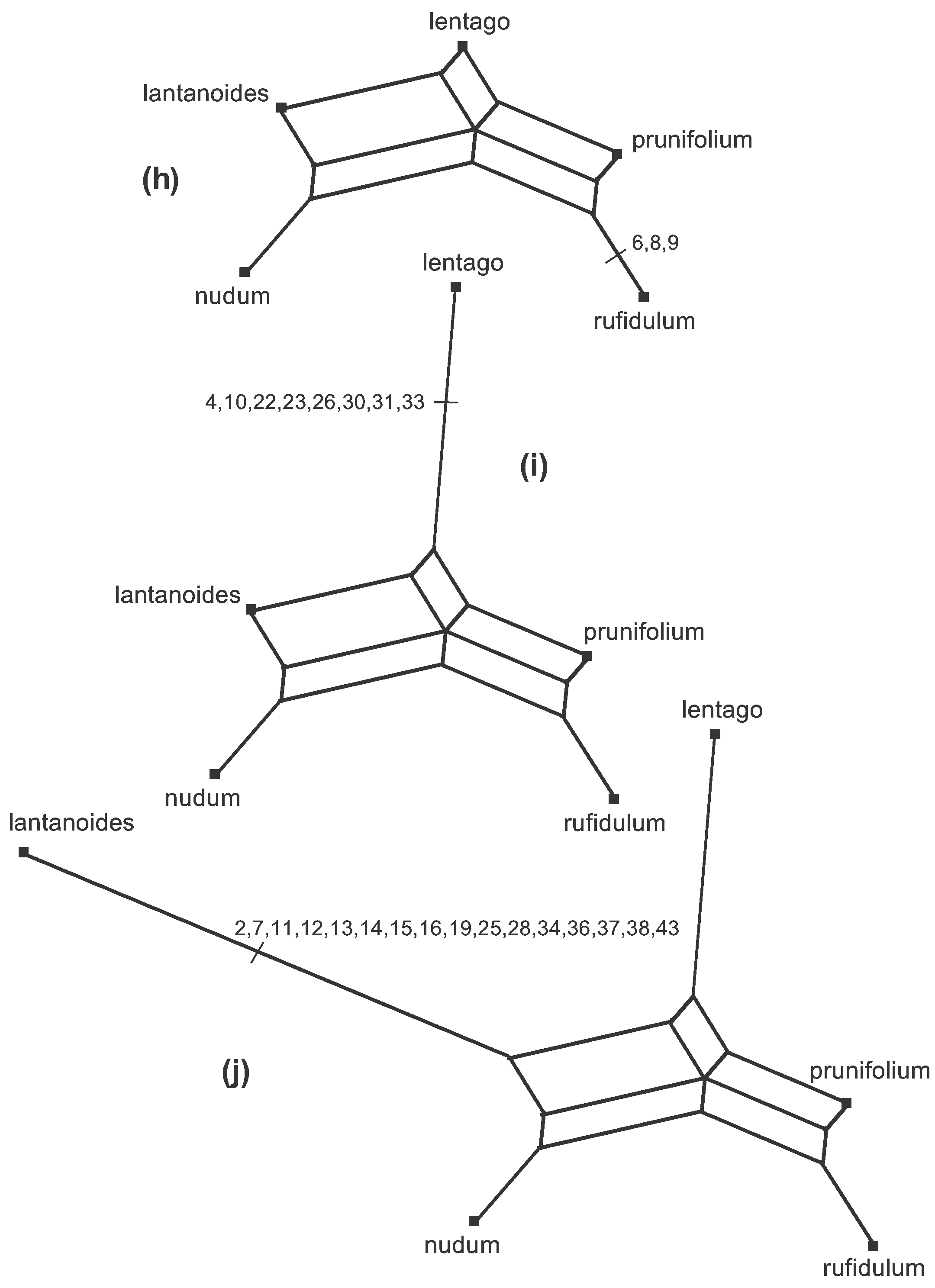
Figure 4. The steps (a–j) to creating a Median Network from the data shown in Figure 2. Note that the characters can be used in any order, so that the order of the steps shown here is arbitrary.

There are 9 data patterns and so there are 9 steps from the initial arrangement (a–j) to creating the network. At each step an edge (or set of parallel edges) is added to the growing network, representing one of the data patterns. The characters involved at each step are marked on the appropriate branch at each step in the Figure. The length of each edge in the Figure is proportional to the number of characters defining (or supporting) that edge.

So, the edge in 4(b) is the first one created, representing the fact that the character states of characters 1, 5, 20, 35 and 39 split the sequences into two groups—the length of the edge represents the five character-state differences between the two groups. Edges are added (in any order) representing the other possible character-state differences, thus creating smaller and smaller groups, until each taxon is in a group of its own.

At step 4(c) the new groups formed are compatible with the two existing groups, in the sense that the new prunifolium-rufidulum group is a subset of an existing group. Therefore, the new edge to be added simply splits that group.

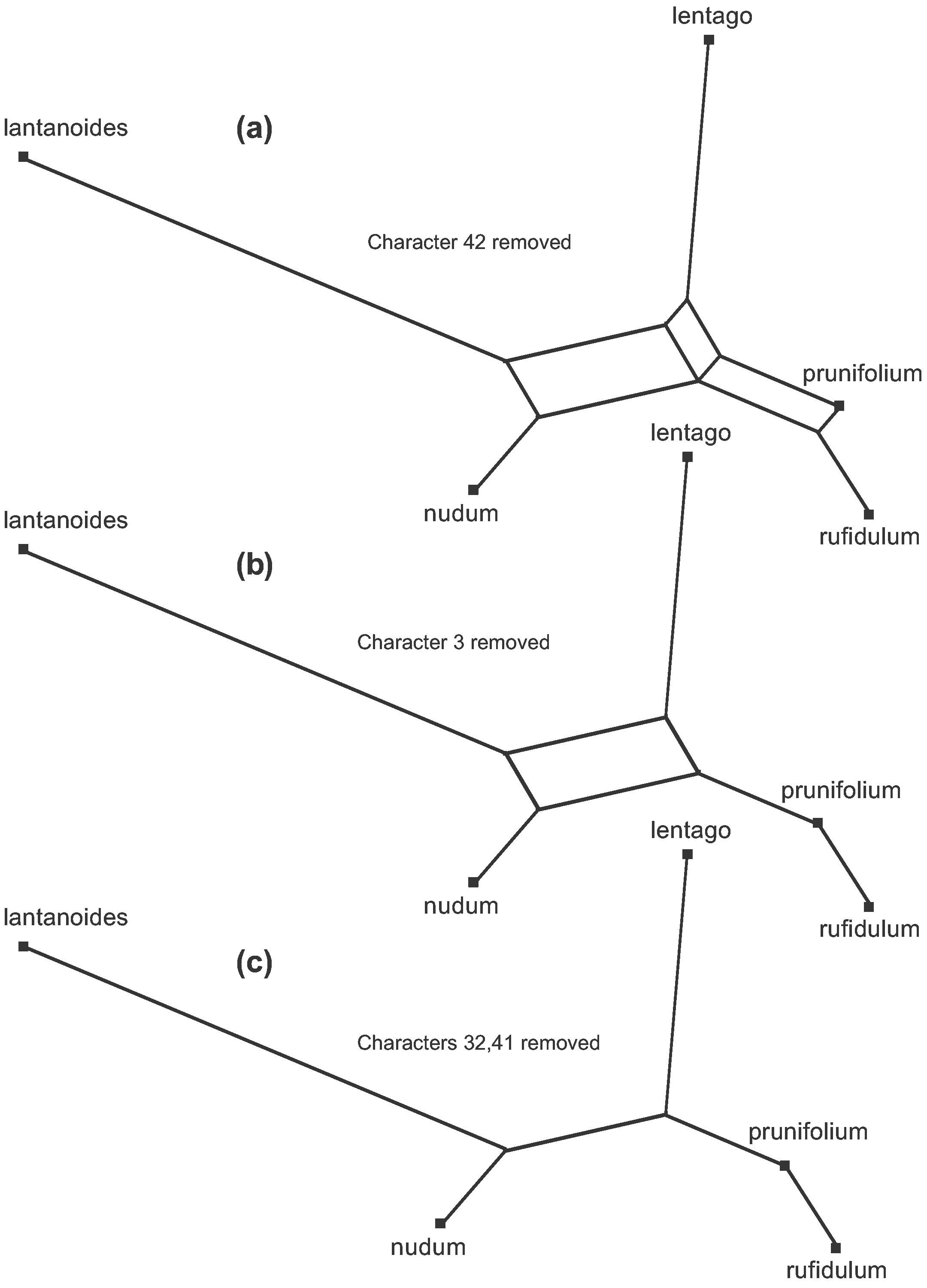
However, at step 4(d) there is a conflict between the two new groups being formed and the three groups that exist at step 4(c). In order to put lantanoides and lentago in a group together in 4(d) when they are in different groups in 4(c), a pair of edges needs to be added rather than a single edge—each new edge originates in a different group. Thus, characters 32 and 41 are represented by two edges rather than one. Note that characters 1, 5, 20, 35 and 39 are now represented by a pair of parallel edges, as well. The same thing happens at steps 4(e) and 4(f)—a set of parallel edges appears rather than a single edge, each one originating in a different pre-existing group. So, both characters 3 and 42 are represented by three edges; and so too are characters 1, 5, 20, 35 and 39, characters 32 and 41, and characters 17, 18, 27 and 29.

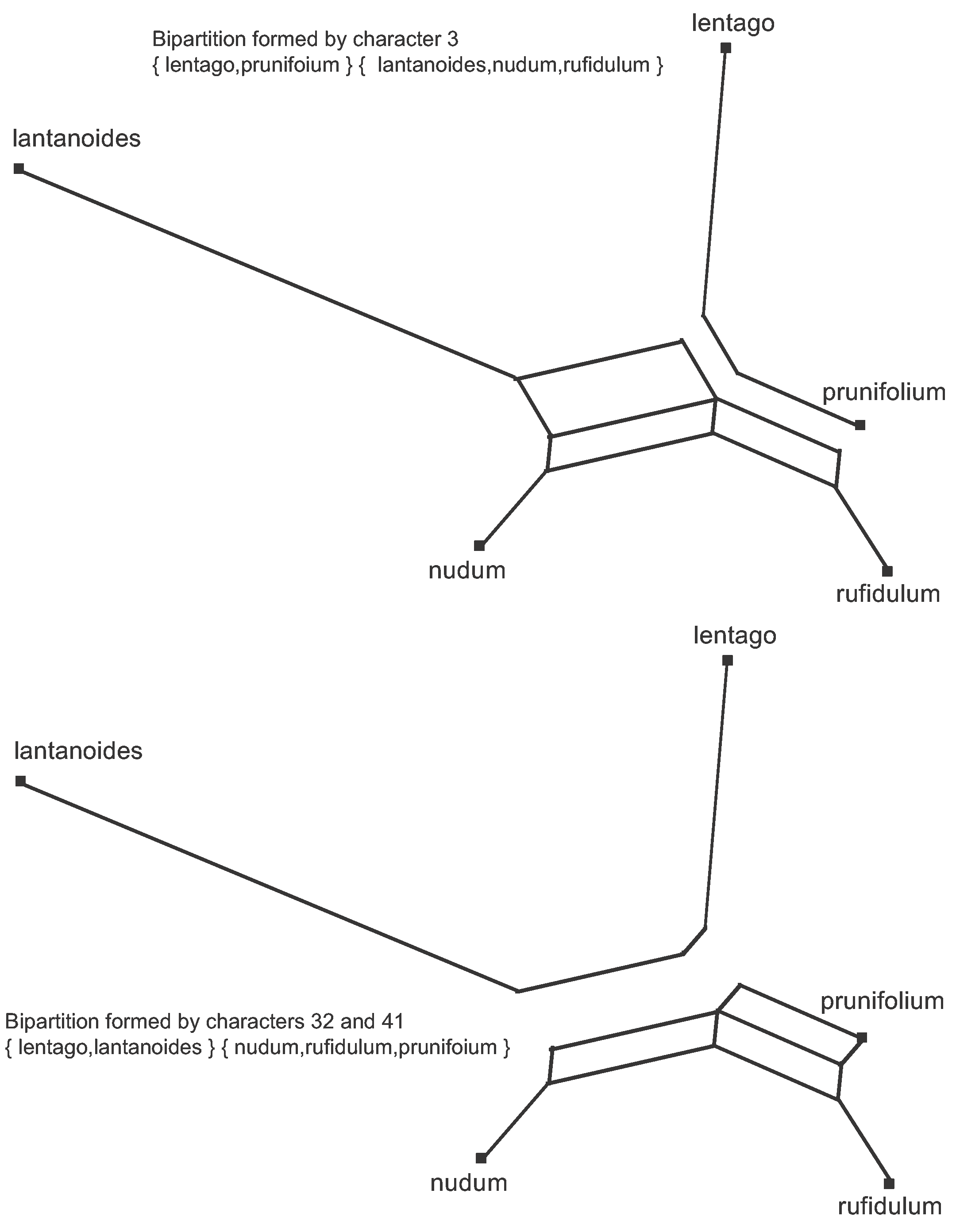
Since the data are binary, every character splits the sequences into two groups, each group being defined by its shared nucleotides. We say that each nucleotide position forms a bipartition of the sequences; and it is the combinations of these bipartitions that form the 9 data patterns. The median network thus displays all of the bipartitions. This is illustrated in Figure 5 for two of the bipartitions.

Figure 5. The bipartitions formed by two of the Viburnum character patterns. One set of parallel edges is removed from the Median Network to show each bipartition.

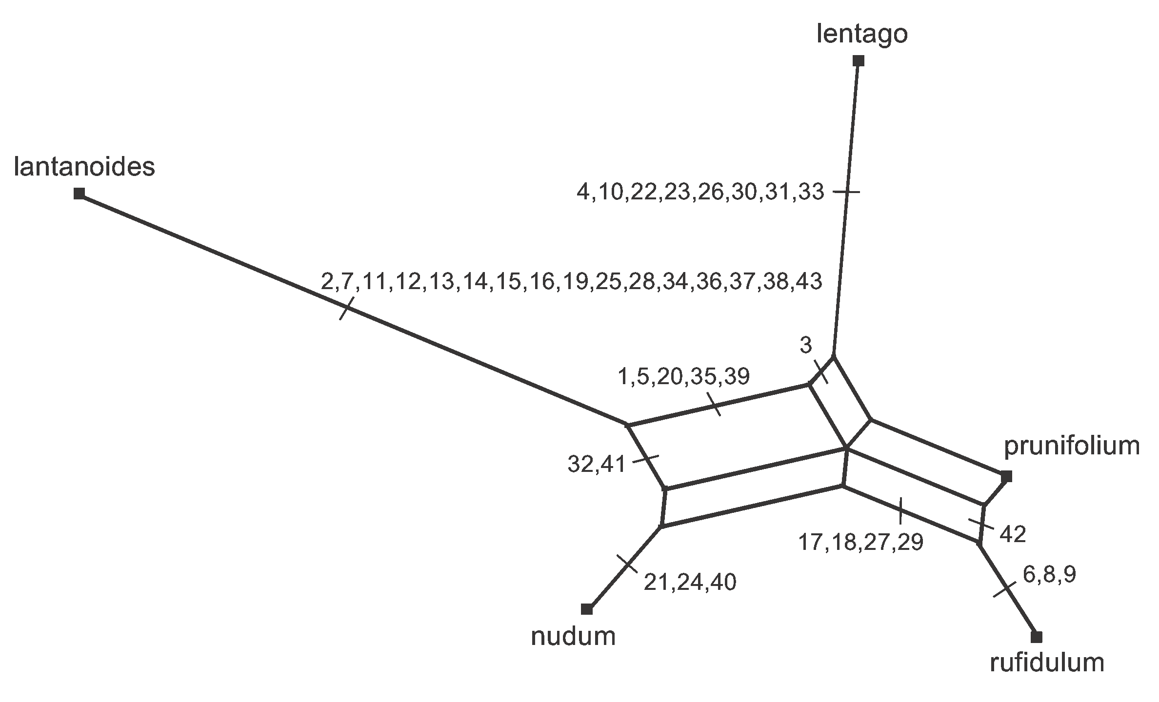
Note that a splits graph is actually a separation network, in the sense that the lines separate the sequences into groups rather than connecting sequences together. This is obvious from the way the graph is formed, as shown in Figure 4. In Figure 6, all of the characters are marked on the branch representing their bipartition. Clearly, the data are not very tree-like in this example, as the characters show a great deal of conflict. Instead there is a network of reticulating interconnections. Also, note that there is no pattern that is unique to prunifolium, and hence there is no edge separating it from the main part of the network.

Figure 6. The Median Network for the Viburnum sequence, showing the edges (or sets of parallel edges) associated with each of the 43 characters.

Trees

If we perform a tree-building analysis of these data then the conflicts among the characters must be resolved in some way. The simplest approach is to use the character weights. For example, if three characters support a particular data pattern and two characters conflict with it, then the three characters would outweigh the two, and the latter pattern would be ignored when building the tree. The tree is thus built solely from the best-supported unconflicting patterns.

This is shown step by step in Figure 7. This figure is also available as an animation (click to open the animation is a new window—the animation loops indefinitely).

There are 5 patterns that conflict pairwise (see Figure 6), and only two of these can be included in the tree. Thus, there are three steps to deriving the tree, each step eliminating one of the conflicting patterns. In order, characters 42, 3, 32 and 41 are deleted, leaving the remaining characters without conflicts. Biologically, characters 3, 32, 41 and 42 are thus treated as homoplasies on the phylogenetic tree rather than homologies.

Figure 7. The steps (a–c) to creating the unrooted Parsimony Tree from the Median Network shown in Figure 6.

Note, that this is now a connection network, in the sense that the lines connect the sequences together rather than separating them.

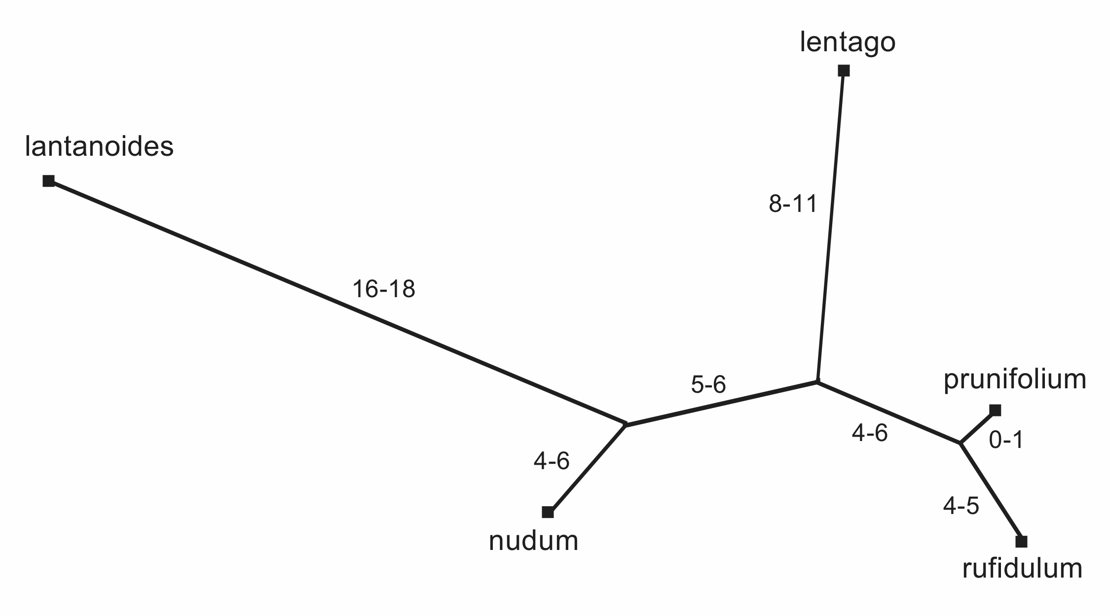
Having derived the topology of the parsimony tree, it is important to note that the relative branch lengths are now somewhat ambiguous. There is only one place where each of the characters can appear on the median network, but there are several ways that the characters can be plotted onto the parsimony tree. This occurs because the conflict between the characters is now hidden rather than displayed, and there are several possible interpretations of where the conflicts occur. This is shown in Figure 8, where the minimum and maximum branch lengths are indicated.

Figure 8. The different possible numbers of characters for each branch of the unrooted Parsimony Tree.

This parsimony analysis displays a subset of the character patterns as an unrooted tree. However, in order to represent a phylogeny the tree must be rooted. The root is necessary in order to determine the direction of genealogical history along the edges, which indicates the historical relationships among the species.

For example, the final tree in Figure 7 does not indicate whether lantanoides and nudum are sisters (which they will be if the root is in the right-hand half of the tree) or whether they are more distant relatives (which they will be if the root is in the left-hand half of the tree).

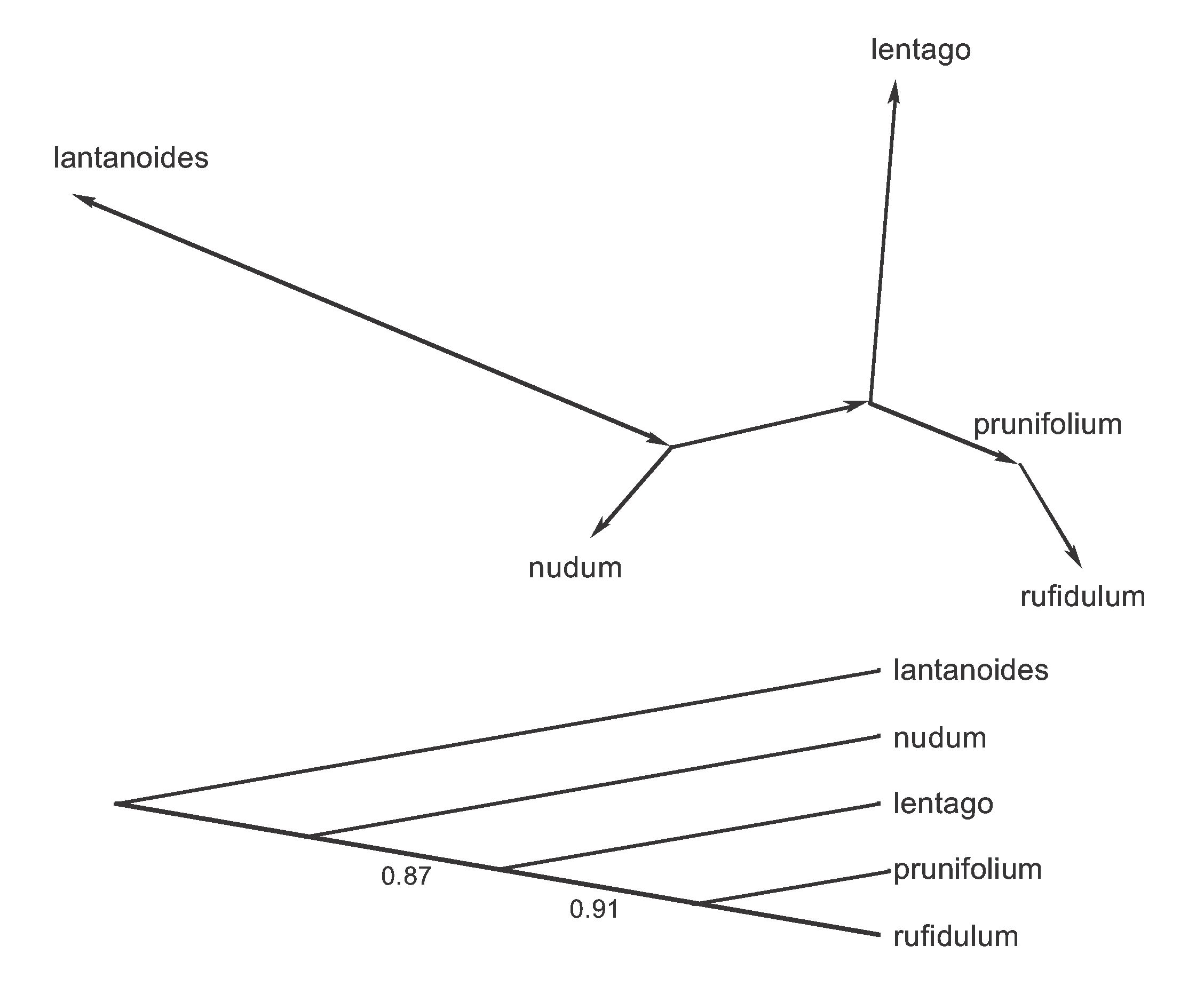
In this instance the root is on the edge connecting lantanoides to the other species, based on outgroup analysis involving other species not used in this dataset. We can draw the rooted Parsimony Tree in either of the two ways shown in Figure 9.

Figure 9. Two illustrations of the rooted Parsimony Tree from the unrooted tree in Figure 8. Bootstrap proportions are shown for the two internal edges of the bottom tree.

Phylogeneticists conventionally draw the tree in the bottom orientation, in which the root is placed at one end of the figure and the edges are implicitly directed away from that point. Mathematicians often use the upper version, in which the edges are explicitly labelled with arrows to indicate their direction away from the root. Note, also, that the bottom version does not have edge lengths proportional to the number of supporting characters (as in the other part of the Figure), but it could have been drawn that way.

The parsimony tree at the bottom of Figure 9 also has bootstrap proportions indicated on it. Note that these are very large (they can range from 0-1), which might seem surprising given the amount of data conflict indicated in Figure 6. It is important to realize that the splits graph and the bootstrap analysis are measuring different things. The splits graph quantifies and displays the amount of conflict that there is in the dataset, whereas the bootstrap analysis quantifies the among of support there is in the data for a tree. That is, each step in the bootstrap analysis forces the data into a tree, thereby eliminating all conflicting data patterns. The splits analysis, on the other hand, does not force the data into any pre-specified model—if there is no conflict in the data then the resulting graph will be a tree, otherwise it will be a reticulating network showing both the location and the nature of the conflict. In this sense, the network analysis is a better data display for EDA than is the tree.

It is also important to note that the same rooting procedure used here cannot be used for a splits graph. To build the tree we first constructed an unrooted tree and then rooted it, but trying to root an unrooted data-display network is inappropriate. In the rooted tree, the nodes all represent inferred ancestors and the directions of the edges represent evolutionary changes between those ancestors. However, this will not be true for the data-display network. For some types of network not all of the nodes will represent ancestors, while for other types of network some of the edges will have an ambiguous direction.

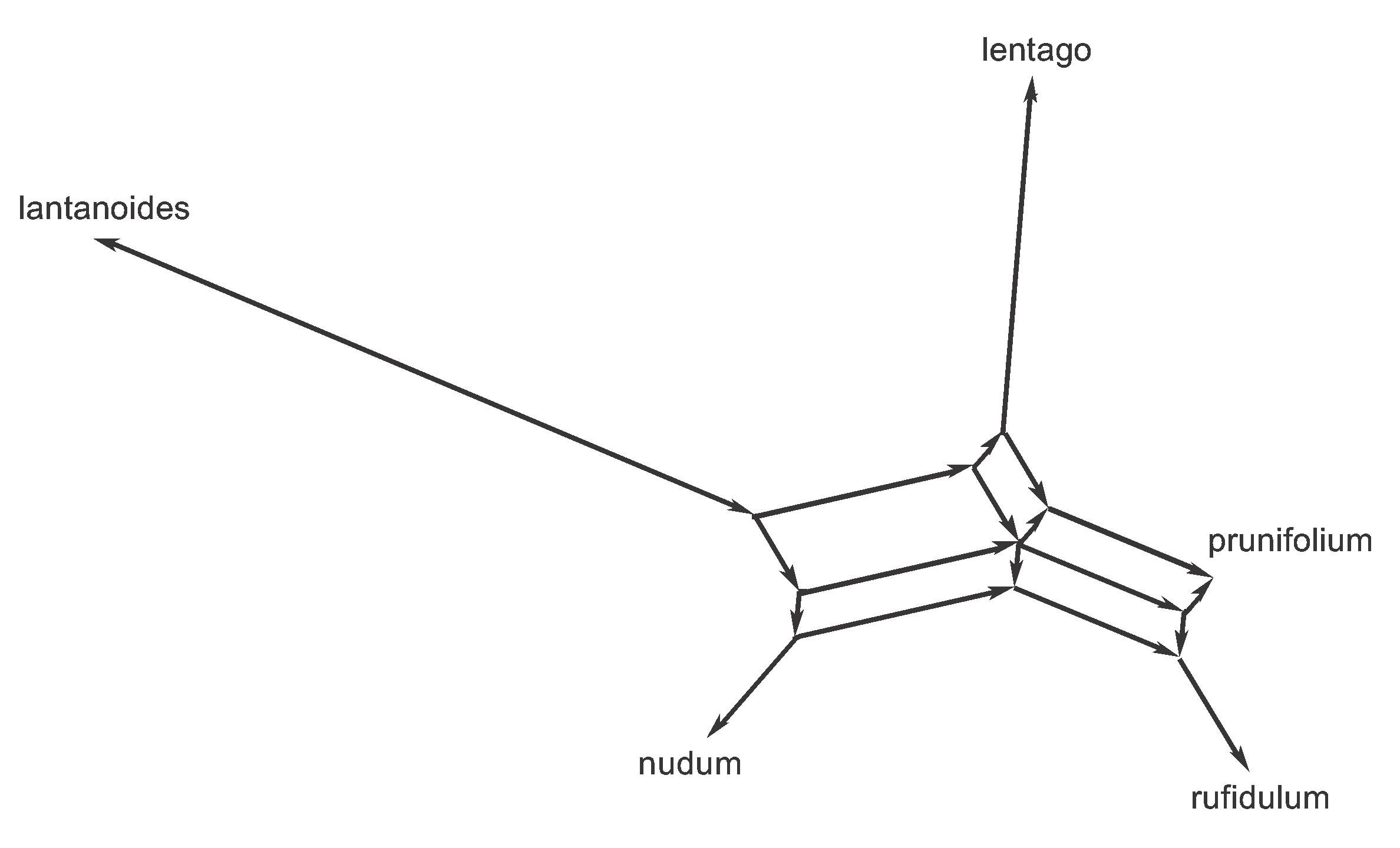
If we do attempt to root the median network (using the outgroup) then we end up with the graph shown in Figure 10. All of the edges have an unambiguous direction (as they always will for splits graphs) but not all of the nodes represent ancestors. There are 10 internal nodes, and most of them are there simply to support a corner of one of the parallelograms—that is, they have a mathematical function but not a biological one.

Figure 10. Rooted version of the Median Network shown in Figure 6.

Other Networks and Trees

Obviously, the dataset used here is very simple. Technically, it has binary data that are only ever pairwise incompatible. Larger datasets will rarely meet these two criteria, so that the data analysis becomes much more complicated. There are many network methods that have been developed it deal with these complexities, most of which have been implemented in computer programs.

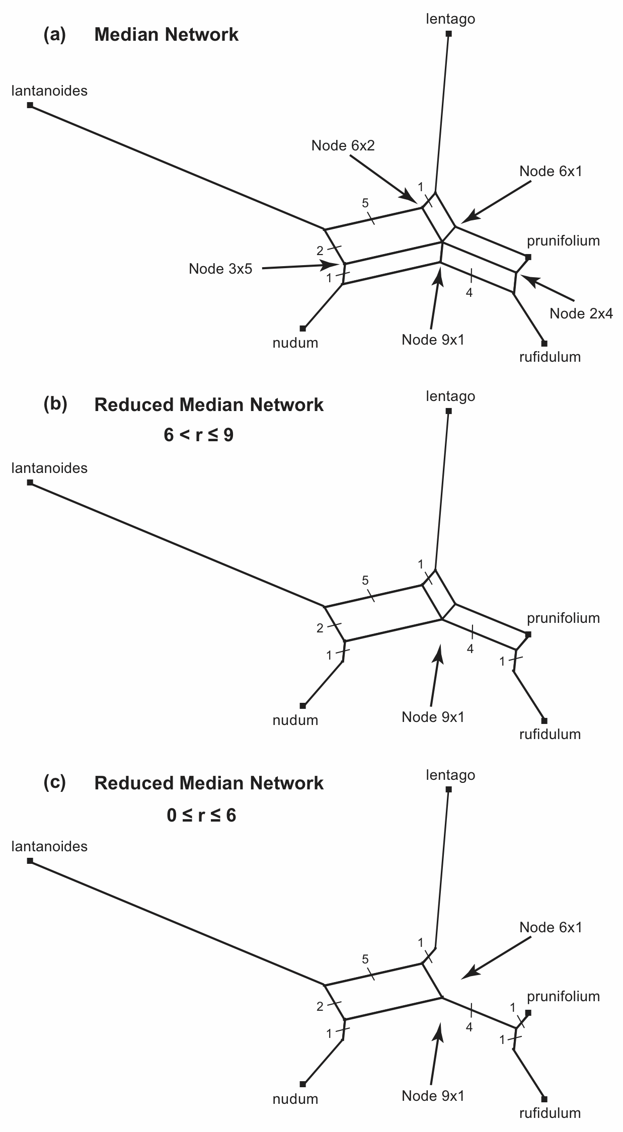
For example, the median network is often far too complex to be of much use as a representation of the data. Therefore, strategies have been developed to produce networks that reduce this complexity. One possible strategy is to start with the median network and then try to simplify it to some specified degree. Another strategy is to to start with a simple network and then add complexity to it to some specified degree. We will look at an example of both of these here.

For the median network shown above, the reticulated part of the network consists of five nodes that support a pair of boxes each, as labelled in Figure 11(a). If any of these nodes is deleted then a pair of boxes would disappear. Thus, we could simplify the network by deleting one or more of these five nodes. If we do this then we have a Reduced Median Network. (Note that there is also one node that supports five boxes; but, we do not need to concern ourselves about nodes with more than a pair of boxes, because these will automatically be reduced as a result of dealing with the pairs.)

Figure 11. The different possible Reduced Median Networks that can be derived from the Median Network shown in Figure 6. The number of characters for each edge is shown.

Each pair of boxes has a certain size, measured in numbers of characters. For example, the bottom pair of boxes is a total of 9 characters wide and 1 character deep (5 of the characters are in the box to the left of the node and 4 are in the box to the right). It is these box sizes that determine which nodes get deleted to produce the reduced median network. We specify this as a "reduction parameter" (r), which is r = width / depth. So, in Figure 11(a) the values of r are (clockwise from the top): 6/2=3, 6/1=6, 2/4=0.5, 9/1=9, and 3/5=0.6.

If we specify r > 9 for reducing the Median Network, then none of the nodes will be deleted, because the largest r in the example network is r = 9. That is, we would not actually reduce the median network.

However, if r ≤ 9 then Node 9x1 will be deleted, as shown in Figure 11(b). Note that what was a set of three parallel edges is now reduced to two edges, which are isolated from each other—these edges are then merged with their adjacent edges. This is one possible reduced median network for the original median network.

If r > 6 then this will be the only node deleted. However, if we specify r ≤ 6 then both Node 9x1 and Node 6x1 will be deleted, as shown in Figure 11(c). Furthermore, these will be the only nodes deleted, because once they have been deleted the network is reduced to a single box, and there are thus no more box pairs. This is the other possible reduced median network for the original median network.

It is important to note that the reduced median network is not necessarily unique for any specified median network—how many there are is determined by the pattern of box pairs; and we use the r parameter to decide which one we will produce. That is, r allows us to decide how much we will simplify the median network.

That is one popular way to simplify a median network. In order to consider another popular method, we first need to introduce an alternative type of tree and network.

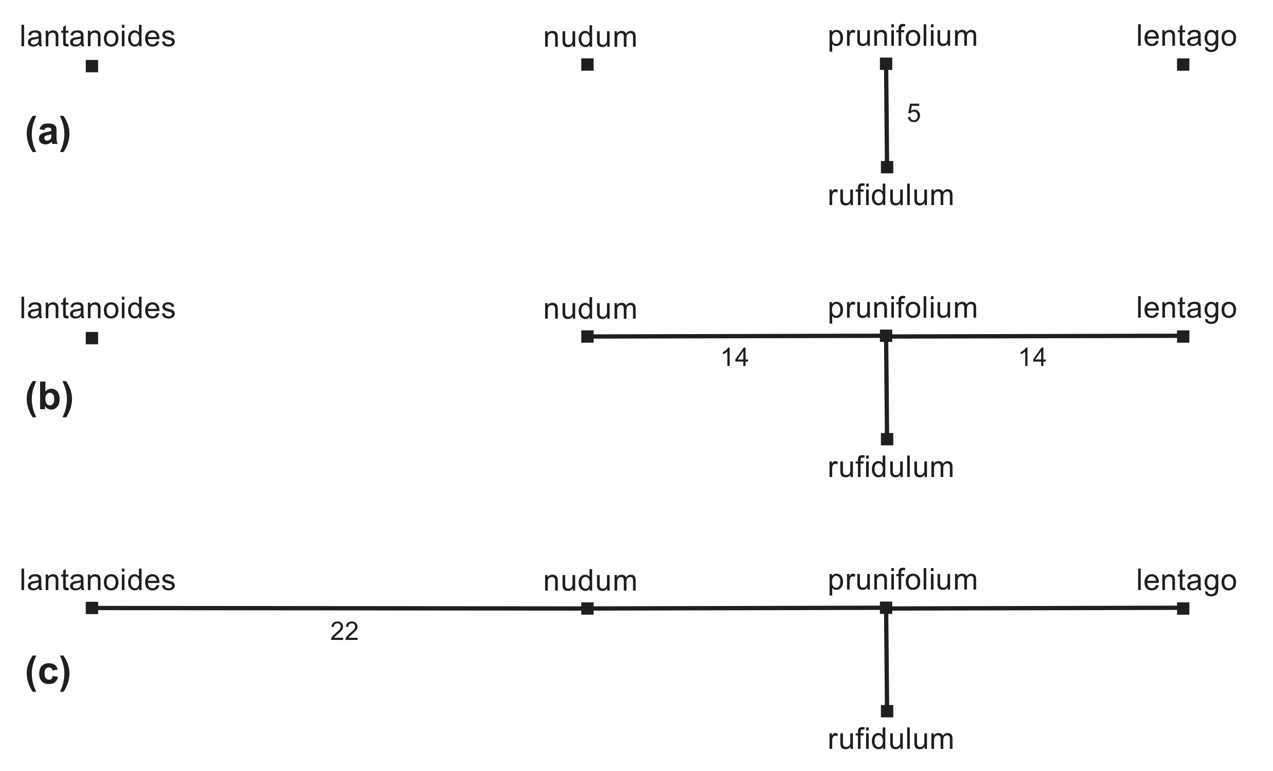
For the Minimum-Spanning Tree the objective is to join the sequences so that the tree is the shortest total length. It is constructed by successively connecting the sequences to each other in order of the number of character differences between them, as shown in Figure 12. This requires only 3 steps in this example, as two of the distances are identical (and are thus added at the same time). In this example there is only one minimum-spanning tree, but when there are several such trees, they are combined into a Minimum-Spanning Network.

Figure 12. The steps in the construction of a Minimum-Spanning Network. The number of characters for each edge is shown.

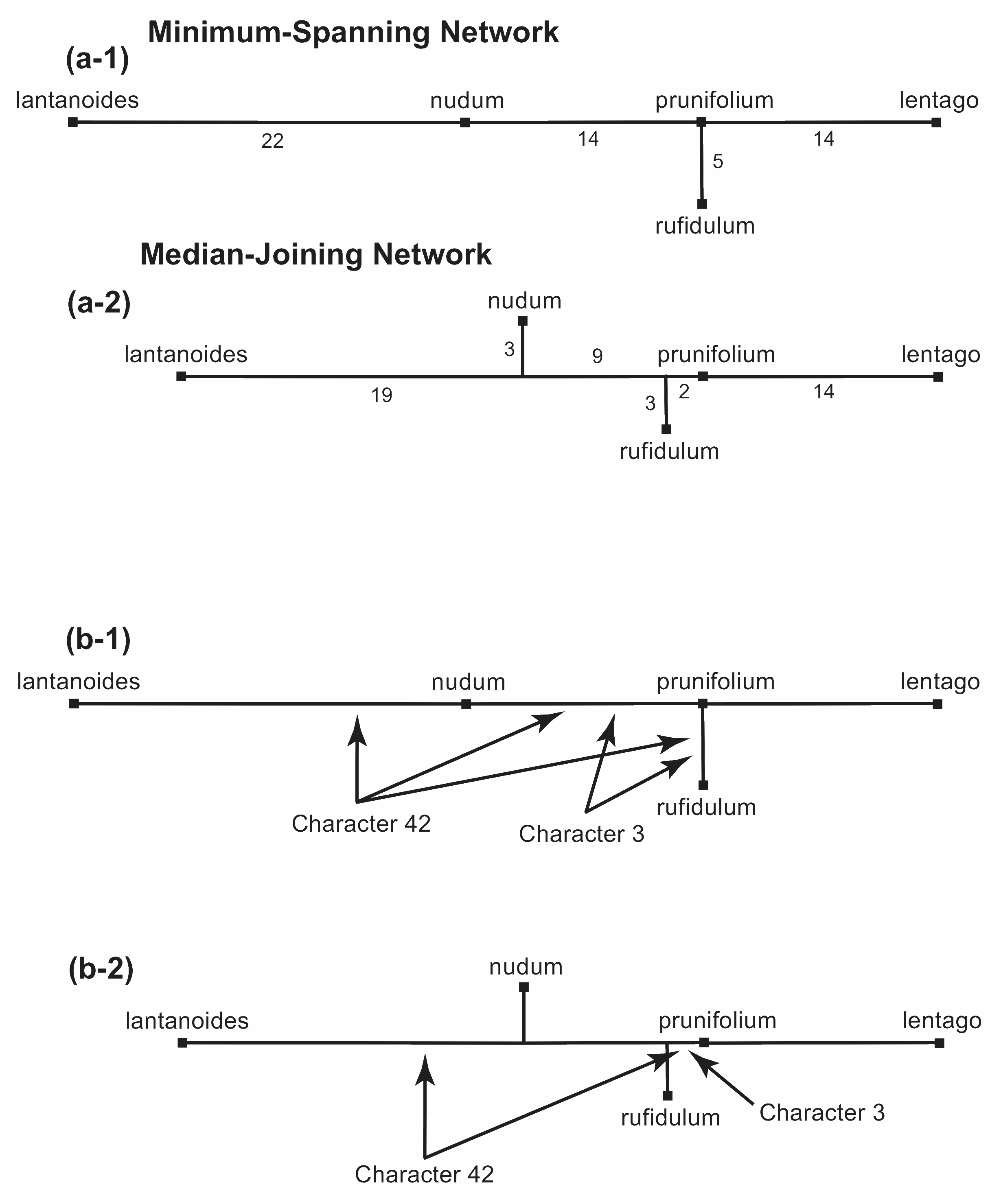
The Median-Joining Network is constructed from the minimum-spanning network (which, in this example, is identical to the minimum-spanning tree). Extra nodes are added to this network in order to shorten the total length, as shown in Figure 13(a). The complexity of the network is specified by a "distance parameter" (ε), which indicates the distance from the sequences within which the new nodes may be added. If ε is large enough then we will end up with the median network.

In Figure 13(a) in the example, the total length of the network is shortened from 55 to 50 by the addition of two extra nodes. Instead of connection rufidulum directly to prunifolium (Figure 13 a-1) it is connected to an extra node (Figure a-2), and the same for nudum, which is no longer connected directly to prunifolium. This still forms a tree in this example, since there are no reticulations.

Figure 13. Construction of a Median-Joining Network from a Minimum-Spanning Network. In (a) the number of characters for each edge is shown. In (b) the location of two different characters is shown.

Each of these extra nodes means that there are some characters that now appear on the network less often. This is illustrated for two of the characters in Figure 13(b). Character 3 appears twice in the minimum-spanning network (b-1) but only once in the median-joining network (b-2), and character 42 appears twice instead of three times.

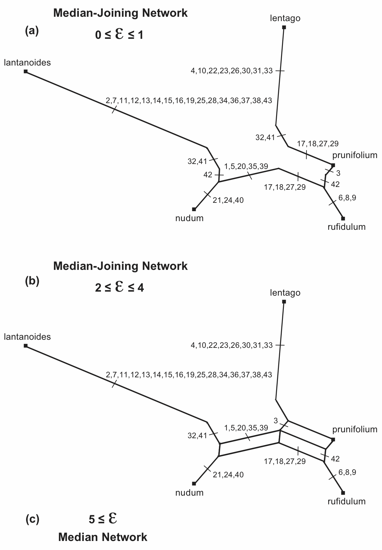
The distribution of the characters themselves is indicated in Figure 14(a), which is identical to Figure 13(a-2) but the tree shape has been drawn to show how the tree edges relate to those in the median network (shown in Figure 6). In particular, the places where characters are duplicated are now obvious. For example, character 3 appears only once in the median-joining network, while character 42 appears twice.

Figure 14. The different possible Median-Joining Networks that can be derived from the Median Network shown in Figure 6. The characters locations are indicated on each edge.

If we specify ε as either 0 or 1, then the median-joining network produced in shown in Figure 14(a), which is thus one possible median-joining network for the original median network. However, if we specify ε as either 2, 3 or 4, then we get the median-joining network shown in Figure 14(b). Here, five more nodes are added (ie. a total of seven), which create reticulations this time, so that it is no longer a tree.

If we specify ε as 5 or greater, then the median-joining network is shown in Figure 14(c), where the remaining three nodes are added that complete the median network. That is, the median-joining network is identical to the median network in this case.

It is important to note that the median-joining network is not necessarily unique for any specified median network—how many there are is determined by the pattern of characters; and we use the ε parameter to decide which one we will produce. That is, ε allows us to decide how much we will simplify the median network.

Finally, the analyses presented so far involve the use of parsimony as the optimality criterion, which leads to a Parsimony Tree and a Median Network (it could also lead to a Parsimony-Splits Network). However, the same thing can also be done using genetic distances as the criterion, which leads to a Neighbor-Joining Tree and a Split-Decomposition Network (it could also lead to a Neighbor-Net network). There are currently no conceptually simple maximum-likelihood or bayesian network methods, although these both exist for trees.

Evolutionary Analysis

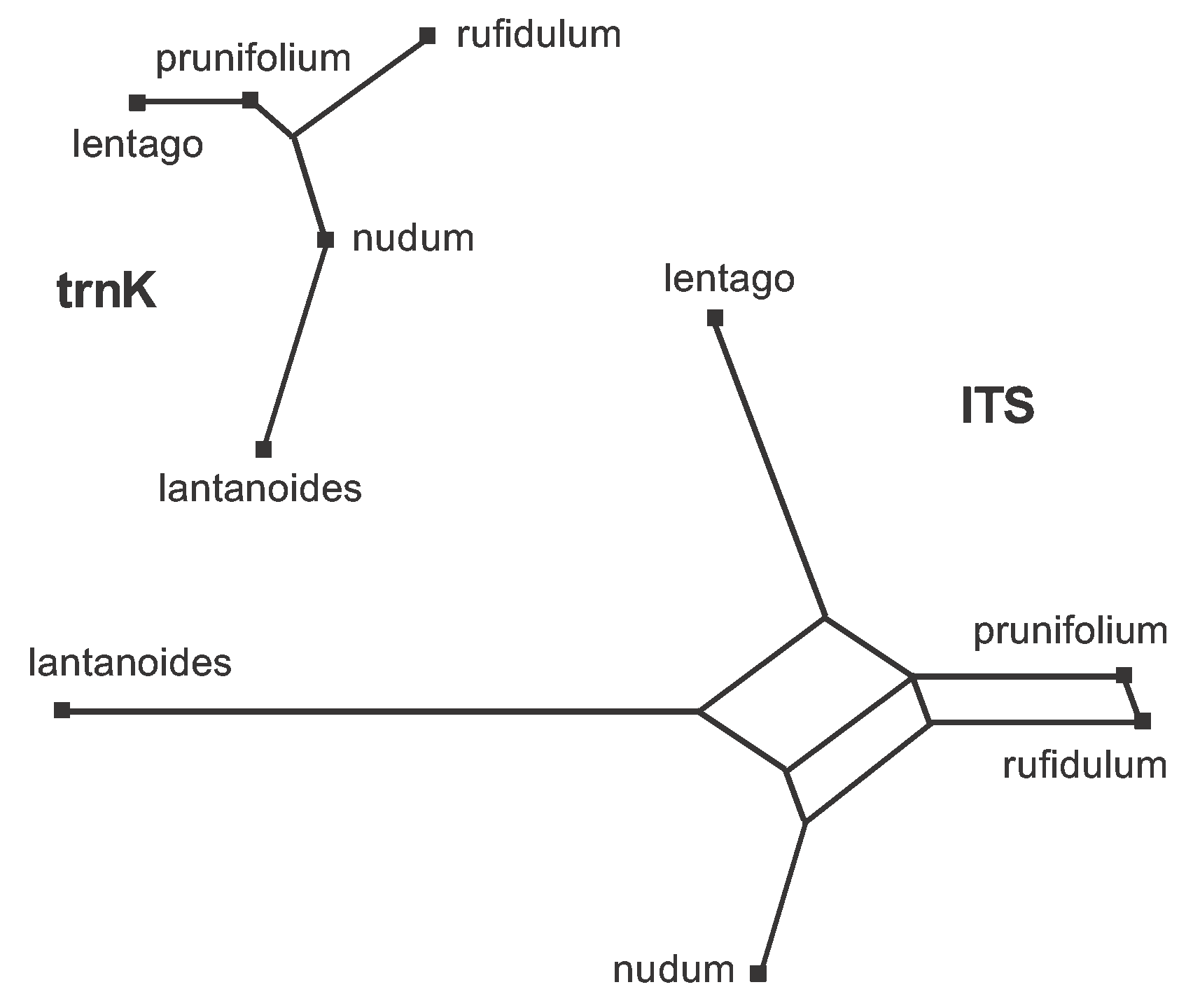
The obvious way to deal with the large amount of data conflict present in the combined dataset (Figure 6) is to analyze the two genes separately. This is easily done using the procedure shown in Figure 4; and the two resulting median networks are shown in Figure 15. You should now be able to work out for yourself which characters should be plotted on each of the edges. Basically, the characters shown in Figure 6 are now distributed across the two gene networks, with characters 1-12 on the trnK network and characters 13-43 on the ITS network.

Figure 15. Median Networks for each of the two genes in the Viburnum dataset. You can compare this with Figure 6 to work out which character(s) support(s) which edge.

Note that the network is a tree for the trnK gene but is still a reticulating network for the ITS gene. This means that there are no conflicting data patterns within the trnK gene. Furthermore, this gene has no pattern that is unique to either prunifolium or nudum. The ITS gene, however, has three conflicting data patterns. Furthermore, {prunifolium,rufidulum} forms a partition in the ITS network but not in the trnK network; and {prunifolium, lentago} forms a partition in the trnaK network but not in the ITS network.

Thus, analyzing the genes separately shows that there are actually two sources of data conflict: (i) within the ITS gene, and (ii) between the two genes. This is one important form of EDA.

We could analyze the within-ITS conflict to see whether data could be explained by recombination. This involves calculating a Recombination Network. Note that this name refers to the mathematical model used not to the biology, although conflict within genes is often caused by recombination. In this example, there seems to be little reason to expect recombination within the ITS region of these plant species. The mathematical analysis is still valid, but you need to be careful of the interpretation—successful application of a mathematical analysis to any particular dataset does not mean that you have correctly identified the underlying biology.

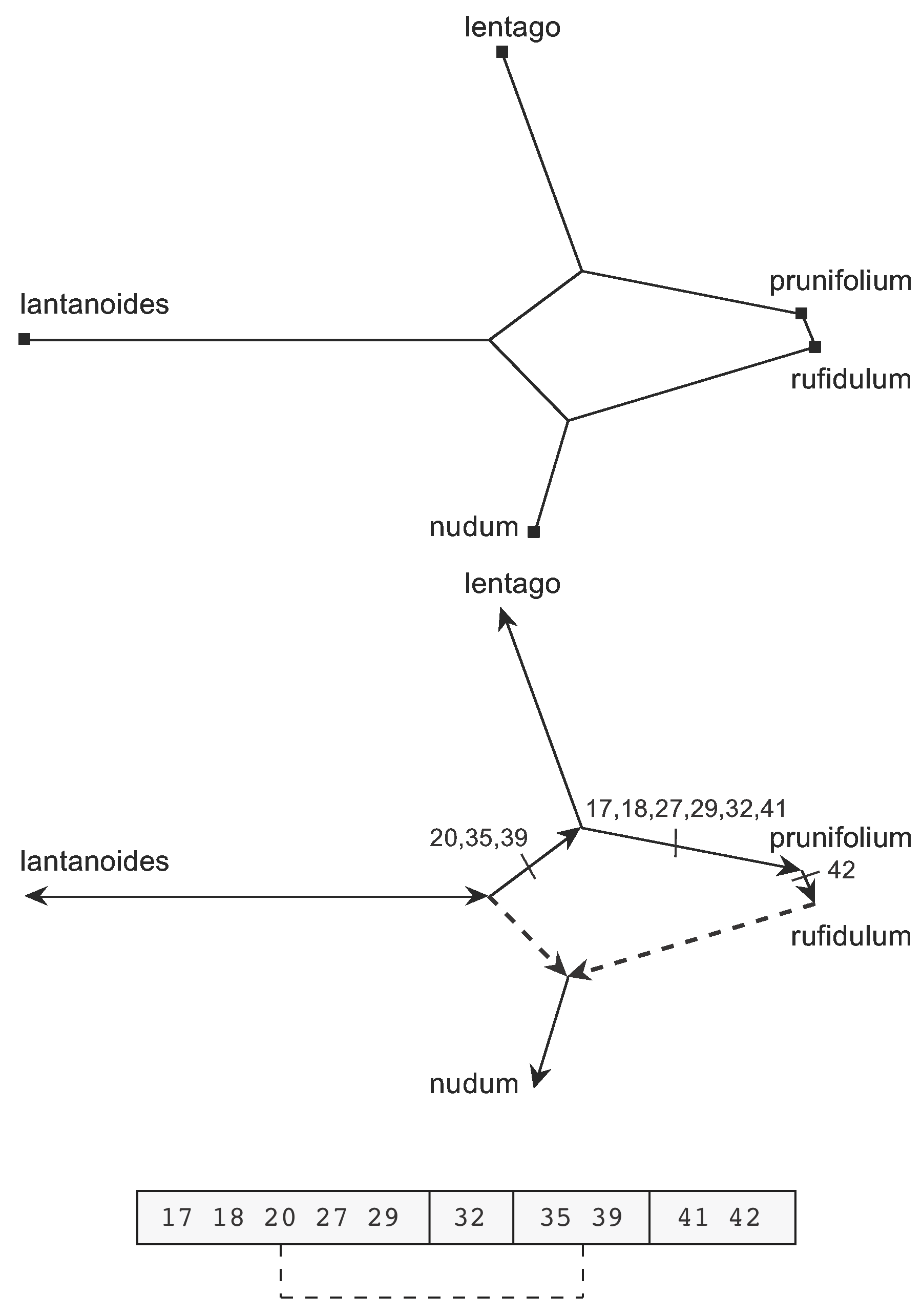
This analysis requires that the characters be in their correct sequence order, unlike any of the other analyses discussed here. The recombination network is produced by (a) simplifying the splits graph to remove the reticulations, and then (b) identifying the recombinant sequence and the crossover (break) points within it.

This is shown in Figure 16. This figure is also available as an animation (click to open the animation is a new window—the animation loops indefinitely).

In this case, the first step is shown at the top of Figure 16. Note that this graph is no longer a splits graph. The second step is shown in the lower part of the Figure, with nudum identified as a recombinant sequence. The directions and character-state changes determined for the non-recombining edges are also shown in the network. This is now a rooted network, rooted in the same manner as for Figure 9, with the root on the edge connecting lantanoides to the other species. The break points are illustrated at the bottom of the Figure, in a schematic version of the sequence with only the relevant character numbers shown.

Figure 16. Steps to creating the Recombination Network for the ITS gene from the Median Network shown in Figure 15.

Note that this example requires a double (simultaneous) crossover, with three break points. The first and third segments shared with rufidulum are recombined with the equivalent segments from lantanoides, so that nudum has a mosaic sequence. Basically, the ancestor of nudum acquires the changed states of all of the characters shown along the arrows in the Figure, and then nudum itself reverts to the ancestral states of characters 17, 18, 20, 27, 29, 35 and 39 via recombination with lantanoides. So, nudum shares the second and fourth gene segments with rufidulum while the first and third segments are shared with lantanoides.

As noted above, this is an unlikely scenario biologically, and so caution is advised.

Moving on, we could analyze the between-gene conflict to see whether the data could be explained by hybridization. Indeed, this was the purpose of the original study, because previous data had suggested that prunifolium might be a hybrid. This involves calculating a Hybridization Network. Once again, this name refers to the mathematical model used not to the biology, although conflict between genes is often caused by hybridization. (Importantly, it could also be caused by horizontal gene transfer.)

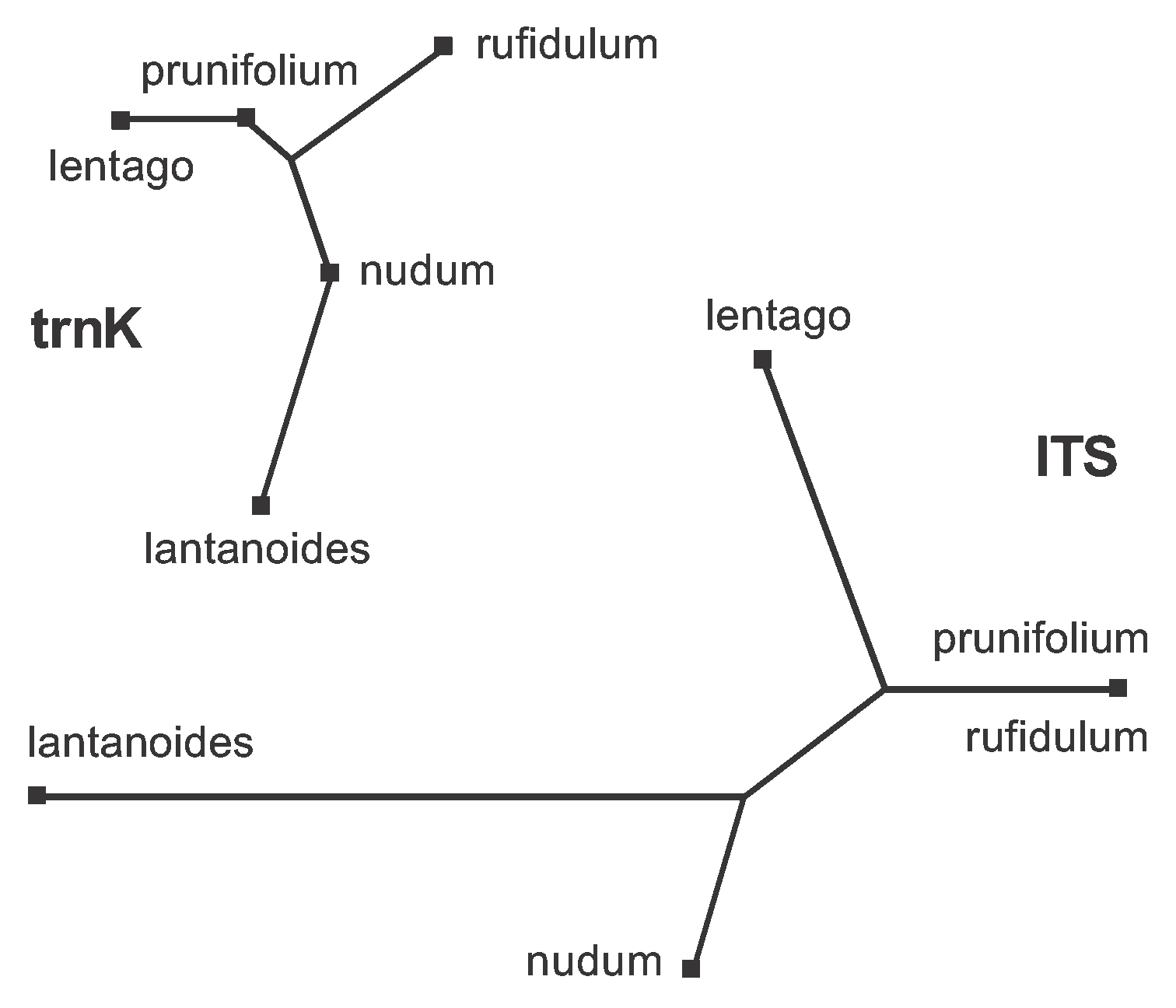
This analysis involves calculating the parsimony trees for both genes. This is trivial for the trnK gene, since the median network is that tree. For the ITS gene we proceed as was done in Figure 7, using the character weights. These two gene trees are shown unrooted in Figure 17.

Figure 17. The two unrooted Parsimony Trees derived from the Median Networks shown in Figure 15.

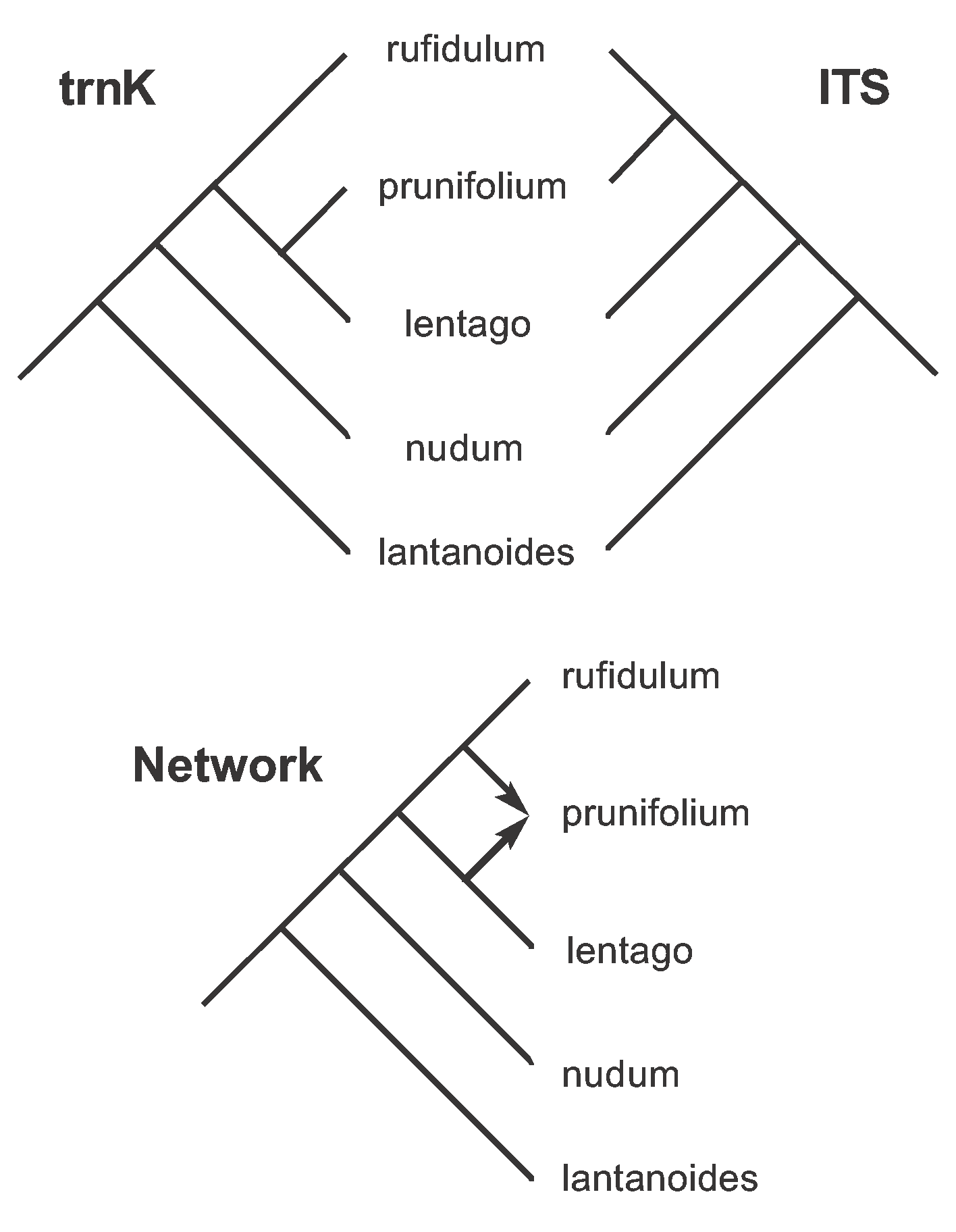
Next, we root these trees as we did for Figure 9, with the root on the branch connecting lantanoides to the other species. The rooted trees are shown in Figure 18. These two trees differ only in the placement of prunifolium: the trnK tree says that prunifolium is the sister to lentago, while the ITS tree says that it is the sister to rufidulum.

Figure 18. The two rooted Parsimony Trees derived from the unrooted trees shown in Figure 17, plus the Hybridization Network derived from these two rooted trees.

The hybridization model says that we should connect prunifolium to both of these tree locations, thus producing the hybridization network. (Technically, we connect the points where the trees differ in rooted-subtree-prune-regraft operations.) This network is also shown in the Figure, clearly indicating that prunifolium is a hybrid between lentago and rufidulum. This is, indeed, exactly what was predicted in the original study, based on the previous biological data.

Note that the hybridization network is produced by (a) removing some of the conflicting data patterns from the network by creating a tree for each gene (so that only the best-supported characters are used in the network), and then (b) displaying the remaining between-tree conflict as reticulations in the network. Also, characters 32, 41 and 42 are still homoplasious with respect to the network (i.e. they cannot be plotted at a single location).

Assumptions

The analyses presented here are based on a set of assumptions, of course. Perhaps the most important one for methods that work directly with characters is that the characters have not been modified multiple times. That is, there have been no "hidden" character changes. For the data presented here, this means that each nucleotide at each alignment position has not been subject to ultiple substitutions.

However, some of the analyses also require that the data be binary. That is, there are no more than two character states for each character. This implies that each character has been modified only once during the evolutionary history of the organisms being studied. For nucleotide data this is called the "infinite sites model" of substitution.

Summary

In this primer I have shown the direct connection that exists between characters and networks, and between the different types of networks. The basic networks are derived from the patterns in the character data; and many of the other network and tree types can be derived from simple network presentations of those patterns.

I have illustrated the importance of EDA in phylogenetics. In the example used, there are many conflicting patterns in the data, and this needs to be taken into account when interpreting the biology, after performing the mathematical analyses.

I have also demonstrated the analysis of suspected hybridization and recombination in a dataset. The recombination analysis is performed on the ordered character data, while the hybridization analysis combines trees derived from those data. Normally, such analyses cannot be performed by hand, due to their mathematical complexity.

Further Reading

Huson D.H., Bryant D. (2006) Application of phylogenetic networks in evolutionary studies. Molecular Biology and Evolution 23: 254–267.

Huson D.H., Rupp R., Scornavacca C. (2011) Phylogenetic Networks: Concepts, Algorithms and Applications. Cambridge University Press, Cambridge.

Huson D.H., Scornavacca C. (2011) A survey of combinatorial methods for phylogenetic networks. Genome Biology and Evolution, 3: 23–35.

Morrison D.A. (2005) Networks in phylogenetic analysis: new tools for population biology. International Journal for Parasitology 35: 567–582.

Morrison D.A. (2010) Using data-display networks for exploratory data analysis in phylogenetic studies. Molecular Biology and Evolution 27: 1044–1057.

Morrison D.A. (2011) Introduction to Phylogenetic Networks. RJR Productions, Uppsala.